Indexes for Joins on Oracle
- kyle Hailey
- Mar 23, 2020
- 11 min read

Looking at ways to programmatically analyze explain plans to see if adding indexes would help.
The analysis is straight forward for for full table scans with strong predicate filters. If there is a strong predicate filter on an explain plan node with a full table scan then it’s a good candidate for an index.
Now a similar situation exists for a join.
Again if the join has a strong predicate filter on a full table scan, that is a candidate.
On the other hand when the actual join fields look like they will benefit from an index, it’s less obvious.
In the queries below T1 and T2 have the same data.
Here is the query
select  max(t1.data) from  t1, t2
where
      t1.id = t2.id
   and t1.clus   = 1  ;
First we try with no indexes.
Then we try with an index on the predicate filter on T1.
Then we add a index on the join column on T2.
The idea being that we should see performance improvements at the addition of each index so that the final efficient path uses the predicate filter index on T1 returning a small amount of rows then drive into T2 with those small amount of rows using the index on T2 join field via an NL join.
The surprising thing is that a HJ that simply hashes values from the predicate filtered rows from T1 and driving into the hash result with all the rows from T2 is just efficient and we don’t have to maintain the index on the t2 join column! It surprising to me. Sure HJs are cool, but I always thought of them as just in time indexes (ie the hashed result) which is work that could be avoid by having an index supporting an NL join and not having to recreate the hash result every query execution. (I’ll have to do some load testing to see what the actual impact of the NL vs HJ query on total database resource usage and load).
Simply adding an index on T1 filter column gets us a HJ that is just as efficient as having a NL using the T2 join field but in the case of the HJ we don’t have to maintain the T2 join column filter.
There is a strong predicate filter on T1.clus ( called “clus” because the values a clustered, we can look non-clustered later, i.e. the same query but using the “val” column which is not clustered)
In the queries below, a NL driving on T1 rows after the predicate filter into T2 using an index on the join, is efficient.
But the HJ , hashing T1 after predicate filter and driving into the hash with all the rows from T2 is surprisingly (to me) as efficient or more efficient).
First example will start with out any index usage.
Create test data:
drop table seed;
create table seed as
select rownum n from dual connect by level <= 1e6
;

drop table t1;
drop table t2;
create table t1 (
    id  int,
    clus int,
    val int,
    data VARCHAR(40)
 );

 insert into t1 (
    id, clus , val, data
)
 select
 n,
 trunc(n/100),
 mod(n,10000),
dbms_random.string('U',dbms_random.value(2,7))
from seed;


select count(*) from t1 where clus = 1;
100
select count(*) from t1 where val = 1;
100

create table t2 as select * from t1;

alter session set Statistics_level=all;
set timing on;
The following 3 examples will use full table scans on both tables.
( I use ” + 0 ” to turn indexes off so I don’t have to drop and recreate for demo since I’ve actually already created the indexes before running these queries )
The first NL below is slower than the next HASH join because the NL has to read the full table T2 for every row in T1 resulting in 300K+ buffer accesses (100 rows after T1 filter time ~3000 buffers per row ).
NL
For every row from T1 (which is all rows from T1 where t1.clus =0 , which is 100 rows)
Look up that row in T2 (T2 doesn’t have an index so we do a full table scan or each 100 rows from above
-> 6.83 secs
The HASH just has to read T2 once (3K+ buffer accesses) and look up each of those rows in a hash of T1 , still a lot of rows ( should be 1M, i.e. all the rows in T2 which is what the estimate says, but actual says 1212 which I don’t understand).
HJ
hash T1 (1000 rows)
look up every row from T2 (1M) in hash of T1
-> 0.09 sec
Hashing T2 instead of T1 is a lot more memory, 50M instead of 1.5 M and takes longer even though its much less look ups from the filter on T1 (only 100).
HJ
hash T2 (1M rows, a good bit of work)
for every row from T1 (100 rows after filter) look them up in hash of T2
-> 0.32 sec
select  /*+ leading(t1 t2)  use_nl(t2) */ max(t1.data) from  t1, t2
where
      t1.id = t2.id  + 0
   and t1.clus + 0  = 1  ;
select * from table(dbms_xplan.display_cursor(null,null,'ALLSTATS LAST'));

--------------------------------------------------------------------------------------
| Id  | Operation	    | Name | Starts | E-Rows | A-Rows |   A-Time   | Buffers |
--------------------------------------------------------------------------------------
|   0 | SELECT STATEMENT    |	   |	  1 |	     |	    1 |00:00:06.83 |	 328K|
|   1 |  SORT AGGREGATE     |	   |	  1 |	   1 |	    1 |00:00:06.83 |	 328K|
|   2 |   NESTED LOOPS	    |	   |	  1 |	  36 |	  100 |00:00:06.83 |	 328K|
|*  3 |    TABLE ACCESS FULL| T1   |	  1 |	  36 |	  100 |00:00:00.07 |	3275 |
|*  4 |    TABLE ACCESS FULL| T2   |	100 |	   1 |	  100 |00:00:06.76 |	 325K|
--------------------------------------------------------------------------------------
   3 - filter("T1"."CLUS"+0=1)
   4 - filter("T1"."ID"="T2"."ID"+0)


select max(t1.data) from  t1, t2
where
    t1.id = t2.id  + 0
   and t1.clus + 0  = 1  ;
select * from table(dbms_xplan.display_cursor(null,null,'ALLSTATS LAST'));

-----------------------------------------------------------------------------------------------------------------
| Id  | Operation	    | Name | Starts | E-Rows | A-Rows |   A-Time   | Buffers |	OMem |	1Mem | Used-Mem |
-----------------------------------------------------------------------------------------------------------------
|   0 | SELECT STATEMENT    |	   |	  1 |	     |	    1 |00:00:00.09 |	3281 |	     |	     |		|
|   1 |  SORT AGGREGATE     |	   |	  1 |	   1 |	    1 |00:00:00.09 |	3281 |	     |	     |		|
|*  2 |   HASH JOIN SEMI    |	   |	  1 |	  36 |	  100 |00:00:00.09 |	3281 |	1753K|	1753K| 1414K (0)|
|*  3 |    TABLE ACCESS FULL| T1   |	  1 |	  36 |	  100 |00:00:00.09 |	3275 |	     |	     |		|
|   4 |    TABLE ACCESS FULL| T2   |	  1 |	1000K|	 1212 |00:00:00.01 |	   6 |	     |	     |		|
-----------------------------------------------------------------------------------------------------------------

Predicate Information (identified by operation id):
---------------------------------------------------

   2 - access("T1"."ID"="T2"."ID"+ 0)
   3 - filter("T1"."CLUS"+ 0=1)


select  /*+ leading(t2 t1) use_hash(t1) max(t1.data) */   max(t1.data)  from  t1, t2
where
    t1.id = t2.id  + 0
   and t1.clus + 0  = 1  ;
select * from table(dbms_xplan.display_cursor(null,null,'ALLSTATS LAST'));

-----------------------------------------------------------------------------------------------------------------
| Id  | Operation	    | Name | Starts | E-Rows | A-Rows |   A-Time   | Buffers |	OMem |	1Mem | Used-Mem |
-----------------------------------------------------------------------------------------------------------------
|   0 | SELECT STATEMENT    |	   |	  1 |	     |	    1 |00:00:00.32 |	6526 |	     |	     |		|
|   1 |  SORT AGGREGATE     |	   |	  1 |	   1 |	    1 |00:00:00.32 |	6526 |	     |	     |		|
|*  2 |   HASH JOIN	    |	   |	  1 |	  36 |	  100 |00:00:00.32 |	6526 |	  50M|	9345K|	 49M (0)|
|   3 |    TABLE ACCESS FULL| T2   |	  1 |	1000K|	 1000K|00:00:00.03 |	3251 |	     |	     |		|
|*  4 |    TABLE ACCESS FULL| T1   |	  1 |	  36 |	  100 |00:00:00.08 |	3275 |	     |	     |		|
-----------------------------------------------------------------------------------------------------------------
Add an index on the predicate filter:
create index t1_clus on t1 (clus);
And we get a much faster hash join access as we access a lot less buffers on T1.
NL driving from T1 still has to do a full table scan on T2 for every row so is slow.
select max(t1.data) from  t1, t2
where
    t1.id = t2.id  + 0
   and t1.clus    = 1  ;
select * from table(dbms_xplan.display_cursor(null,null,'ALLSTATS LAST'));


--------------------------------------------------------------------------------------------------------------------------------
| Id  | Operation			      | Name	| Starts | E-Rows | A-Rows |   A-Time	| Buffers |  OMem |  1Mem | Used-Mem |
--------------------------------------------------------------------------------------------------------------------------------
|   0 | SELECT STATEMENT		      | 	|      1 |	  |	 1 |00:00:00.01 |      10 |	  |	  |
|   1 |  SORT AGGREGATE 		      | 	|      1 |	1 |	 1 |00:00:00.01 |      10 |	  |	  ||
|*  2 |   HASH JOIN SEMI		      | 	|      1 |    100 |    100 |00:00:00.01 |      10 |  1753K|  1753K| 1408K (0)|
|   3 |    TABLE ACCESS BY INDEX ROWID BATCHED| T1	|      1 |    100 |    100 |00:00:00.01 |	4 |	  |	  ||
|*  4 |     INDEX RANGE SCAN		      | T1_CLUS |      1 |    100 |    100 |00:00:00.01 |	3 |	  |	  ||
|   5 |    TABLE ACCESS FULL		      | T2	|      1 |   1000K|   1212 |00:00:00.01 |	6 |	  |	  ||
--------------------------------------------------------------------------------------------------------------------------------

Predicate Information (identified by operation id):
---------------------------------------------------

2 - access("T1"."ID"="T2"."ID")
4 - access("T1"."MILLI"=1)


select /*+ leading(t1 t2)  use_nl(t2) */  max(t1.data) from  t1, t2
where
      t1.id = t2.id + 0
   and t1.clus   = 1  ;
select * from table(dbms_xplan.display_cursor(null,null,'ALLSTATS'));

--------------------------------------------------------------------------------------------------------------------
| Id  | Operation			      | Name	| Starts | E-Rows | A-Rows |   A-Time	| Buffers | Reads  |
--------------------------------------------------------------------------------------------------------------------
|   0 | SELECT STATEMENT		      | 	|      1 |	  |	 1 |00:08:14.23 |    2893K|   2892K|
|   1 |  SORT AGGREGATE 		      | 	|      1 |	1 |	 1 |00:08:14.23 |    2893K|   2892K|
|   2 |   NESTED LOOPS			      | 	|      1 |    100 |    100 |00:08:14.23 |    2893K|   2892K|
|   3 |    TABLE ACCESS BY INDEX ROWID BATCHED| T1	|      1 |    100 |    100 |00:00:00.01 |	4 |	 0 |
|*  4 |     INDEX RANGE SCAN		      | T1_CLUS |      1 |    100 |    100 |00:00:00.01 |	3 |	 0 |
|*  5 |    TABLE ACCESS FULL		      | T2	|    100 |	1 |    100 |00:08:14.23 |    2893K|   2892K|
--------------------------------------------------------------------------------------------------------------------
Adding on index on T2.id and allowing the NL driving from T1 to look up rows in T2 by index gets the NL down to about the same as HASH JOIN.
The HJ is on hash of T2 is faster when accessing T1 by it’s index on the predicate filter but still hashing all of T2 slows it down.
I don’t understand why the HJ hashing on T2 is slower when accessing T1 by index instead of full table scan.
drop index t2_id;

create index t2_id on t2 (id);

select /*+ leading(t1 t2)  use_nl(t2) */  max(t1.data) from  t1, t2
where
      t1.id = t2.id
   and t1.clus   = 1  ;
select * from table(dbms_xplan.display_cursor(null,null,'ALLSTATS'));

-----------------------------------------------------------------------------------------------------------
| Id  | Operation			      | Name	| Starts | E-Rows | A-Rows |   A-Time	| Buffers |
-----------------------------------------------------------------------------------------------------------
|   0 | SELECT STATEMENT		      | 	|      1 |	  |	 1 |00:00:00.01 |      17 |
|   1 |  SORT AGGREGATE 		      | 	|      1 |	1 |	 1 |00:00:00.01 |      17 |
|   2 |   NESTED LOOPS SEMI		      | 	|      1 |    100 |    100 |00:00:00.01 |      17 |
|   3 |    TABLE ACCESS BY INDEX ROWID BATCHED| T1	|      1 |    100 |    100 |00:00:00.01 |	4 |
|*  4 |     INDEX RANGE SCAN		      | T1_CLUS |      1 |    100 |    100 |00:00:00.01 |	3 |
|*  5 |    INDEX RANGE SCAN		      | T2_ID	|    100 |   1000K|    100 |00:00:00.01 |      13 |
-----------------------------------------------------------------------------------------------------------

select /*+ leading(t2 t1) use_hash(t1)  */
max(t1.data) from  t1, t2
where
      t1.id = t2.id +1
   and t1.clus = 1  ;
select * from table(dbms_xplan.display_cursor(null,null,'ALLSTATS LAST'));

--------------------------------------------------------------------------------------------------------------------------------------
| Id  | Operation			      | Name	| Starts | E-Rows | A-Rows |   A-Time	| Buffers |  OMem |  1Mem | Used-Mem |
--------------------------------------------------------------------------------------------------------------------------------
|   0 | SELECT STATEMENT		      | 	|      1 |	  |	 1 |00:00:00.22 |    3255 |	  |	  ||
|   1 |  SORT AGGREGATE 		      | 	|      1 |	1 |	 1 |00:00:00.22 |    3255 |	  |	  ||
|*  2 |   HASH JOIN			      | 	|      1 |     78 |    100 |00:00:00.22 |    3255 |    50M|  9345K|   49M (0)|
|   3 |    TABLE ACCESS FULL		      | T2	|      1 |   1000K|   1000K|00:00:00.03 |    3251 |	  |	  ||
|   4 |    TABLE ACCESS BY INDEX ROWID BATCHED| T1	|      1 |    100 |    100 |00:00:00.01 |	4 |	  |	  ||
|*  5 |     INDEX RANGE SCAN		      | T1_CLUS |      1 |    100 |    100 |00:00:00.01 |	3 |	  |	  ||
-------------------------------------------------------------------------------------------------------------------------------
Predicate Information (identified by operation id):
---------------------------------------------------

   2 - access("T1"."ID"="T2"."ID"+1)
   5 - access("T1"."CLUS"=1)

select /*+ leading(t2 t1) use_hash(t1)  */
max(t1.data) from  t1, t2
where
      t1.id = t2.id
   and t1.clus = 1  ;
select * from table(dbms_xplan.display_cursor(null,null,'ALLSTATS LAST'));

--------------------------------------------------------------------------------------------------------------------------------
| Id  | Operation			      | Name	| Starts | E-Rows | A-Rows |   A-Time	| Buffers |  OMem |  1Mem | Used-Mem |
--------------------------------------------------------------------------------------------------------------------------------
|   0 | SELECT STATEMENT		      | 	|      1 |	  |	 1 |00:00:01.25 |    2246 |	  |	  ||
|   1 |  SORT AGGREGATE 		      | 	|      1 |	1 |	 1 |00:00:01.25 |    2246 |	  |	  ||
|*  2 |   HASH JOIN			      | 	|      1 |    100 |    100 |00:00:01.25 |    2246 |    43M|  6111K|   42M (0)|
|   3 |    INDEX FAST FULL SCAN 	      | T2_ID	|      1 |   1000K|   1000K|00:00:00.31 |    2242 |	  |	  ||
|   4 |    TABLE ACCESS BY INDEX ROWID BATCHED| T1	|      1 |    100 |    100 |00:00:00.01 |	4 |	  |	  ||
|*  5 |     INDEX RANGE SCAN		      | T1_CLUS |      1 |    100 |    100 |00:00:00.01 |	3 |	  |	  ||
--------------------------------------------------------------------------------------------------------------------------------

Predicate Information (identified by operation id):
---------------------------------------------------

   2 - access("T1"."ID"="T2"."ID")
   5 - access("T1"."CLUS"=1)
For reference, the order of NL and HJ access and hints

reference
Followup:
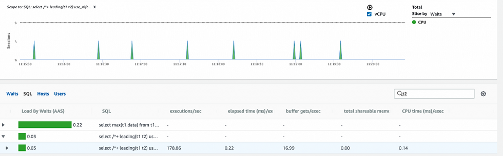
The Hash Join put about 7x (0.22 AAS) as much load on the DB as the next loops (0.03AAS) and both are doing 178 executions/sec.
First Load Chart image with top SQL drill down filters for the efficient HJ version. Th HJ plan is shown here.
--------------------------------------------------------------------------------------------------------------------------------
| Id  | Operation			      | Name	| Starts | E-Rows | A-Rows |   A-Time	| Buffers |  OMem |  1Mem | Used-Mem |
--------------------------------------------------------------------------------------------------------------------------------
|   0 | SELECT STATEMENT		      | 	|      1 |	  |	 1 |00:00:00.01 |      10 |	  |	  |
|   1 |  SORT AGGREGATE 		      | 	|      1 |	1 |	 1 |00:00:00.01 |      10 |	  |	  ||
|*  2 |   HASH JOIN SEMI		      | 	|      1 |    100 |    100 |00:00:00.01 |      10 |  1753K|  1753K| 1408K (0)|
|   3 |    TABLE ACCESS BY INDEX ROWID BATCHED| T1	|      1 |    100 |    100 |00:00:00.01 |	4 |	  |	  ||
|*  4 |     INDEX RANGE SCAN		      | T1_CLUS |      1 |    100 |    100 |00:00:00.01 |	3 |	  |	  ||
|   5 |    TABLE ACCESS FULL		      | T2	|      1 |   1000K|   1212 |00:00:00.01 |	6 |	  |	  ||
--------------------------------------------------------------------------------------------------------------------------------

The second image is the load filtered by the NJ join and here is the explain.
-----------------------------------------------------------------------------------------------------------
| Id  | Operation			      | Name	| Starts | E-Rows | A-Rows |   A-Time	| Buffers |
-----------------------------------------------------------------------------------------------------------
|   0 | SELECT STATEMENT		      | 	|      1 |	  |	 1 |00:00:00.01 |      17 |
|   1 |  SORT AGGREGATE 		      | 	|      1 |	1 |	 1 |00:00:00.01 |      17 |
|   2 |   NESTED LOOPS SEMI		      | 	|      1 |    100 |    100 |00:00:00.01 |      17 |
|   3 |    TABLE ACCESS BY INDEX ROWID BATCHED| T1	|      1 |    100 |    100 |00:00:00.01 |	4 |
|*  4 |     INDEX RANGE SCAN		      | T1_CLUS |      1 |    100 |    100 |00:00:00.01 |	3 |
|*  5 |    INDEX RANGE SCAN		      | T2_ID	|    100 |   1000K|    100 |00:00:00.01 |      13 |
-----------------------------------------------------------------------------------------------------------
The following hash join, which hashes T2, was not as efficient hashing T1 results but it confused me where it looked like using the index on T1 filter was more expensive than not using it. Looks like it’s the other way around in actual load.
Even though skipping the T1 index shows an A-Time of 0.22 and using the T1 Index shows 1.25, when running a concurrent load it looks the opposite.
The first example below avoids the index on T1 and has an AAS of 10.36 and elapsed of 3.7 secs (instead of 0.22 in explain)
The second which uses the index on T1 filter has an AAS of 8.2 and elapsed of 3.1 secs (instead of 1.25 in explain)
Both are executing 2.24 executes/sec.
select /*+ leading(t2 t1) use_hash(t1)  */
max(t1.data) from  t1, t2
where
      t1.id = t2.id +1
   and t1.clus = 1  ;
select * from table(dbms_xplan.display_cursor(null,null,'ALLSTATS LAST'));

--------------------------------------------------------------------------------------------------------------------------------------
| Id  | Operation			      | Name	| Starts | E-Rows | A-Rows |   A-Time	| Buffers |  OMem |  1Mem | Used-Mem |
--------------------------------------------------------------------------------------------------------------------------------
|   0 | SELECT STATEMENT		      | 	|      1 |	  |	 1 |00:00:00.22 |    3255 |	  |	  ||
|   1 |  SORT AGGREGATE 		      | 	|      1 |	1 |	 1 |00:00:00.22 |    3255 |	  |	  ||
|*  2 |   HASH JOIN			      | 	|      1 |     78 |    100 |00:00:00.22 |    3255 |    50M|  9345K|   49M (0)|
|   3 |    TABLE ACCESS FULL		      | T2	|      1 |   1000K|   1000K|00:00:00.03 |    3251 |	  |	  ||
|   4 |    TABLE ACCESS BY INDEX ROWID BATCHED| T1	|      1 |    100 |    100 |00:00:00.01 |	4 |	  |	  ||
|*  5 |     INDEX RANGE SCAN		      | T1_CLUS |      1 |    100 |    100 |00:00:00.01 |	3 |	  |	  ||
-------------------------------------------------------------------------------------------------------------------------------
.

--------------------------------------------------------------------------------------------------------------------------------
| Id  | Operation			      | Name	| Starts | E-Rows | A-Rows |   A-Time	| Buffers |  OMem |  1Mem | Used-Mem |
--------------------------------------------------------------------------------------------------------------------------------
|   0 | SELECT STATEMENT		      | 	|      1 |	  |	 1 |00:00:01.25 |    2246 |	  |	  ||
|   1 |  SORT AGGREGATE 		      | 	|      1 |	1 |	 1 |00:00:01.25 |    2246 |	  |	  ||
|*  2 |   HASH JOIN			      | 	|      1 |    100 |    100 |00:00:01.25 |    2246 |    43M|  6111K|   42M (0)|
|   3 |    INDEX FAST FULL SCAN 	      | T2_ID	|      1 |   1000K|   1000K|00:00:00.31 |    2242 |	  |	  ||
|   4 |    TABLE ACCESS BY INDEX ROWID BATCHED| T1	|      1 |    100 |    100 |00:00:00.01 |	4 |	  |	  ||
|*  5 |     INDEX RANGE SCAN		      | T1_CLUS |      1 |    100 |    100 |00:00:00.01 |	3 |	  |	  ||
--------------------------------------------------------------------------------------------------------------------------------
.


Comments